Essentials of Machine Learning Algorithms
广义而言,机器学习算法分三类 1.监督学习 工作原理:算法从一组给定的预测因子(独立变量)来预测目标/结果变量(或因变量),使用这些变量集生成映射输入到期望输出的函数,不断训练直到模型达到训练数据所需的精度水平。常见算法有:回归(Regression)、决策树(Decision Tree)、随机森林(Random Forest)、KNN、逻辑回归(Logistic Regression)等。
2.无监督学习 工作原理:算法中没有任何目标或结果变量要预测/估计,而是用于不同群体的种群聚集,广泛应用于不同群体的细分。常见算法有:关联规则算法(Apriori algorithm)、K-means。
3.增强学习 工作原理:算法中,机器被训练来做出特定的决定,通过反复试验不断训练机器,机器从过去的经验中学习,捕捉最好的知识以做出准确的决策。常见算法有:马尔科夫决策过程(Markov Decision Process)。
常用机器学习算法 1.线性回归 - Linear Regression
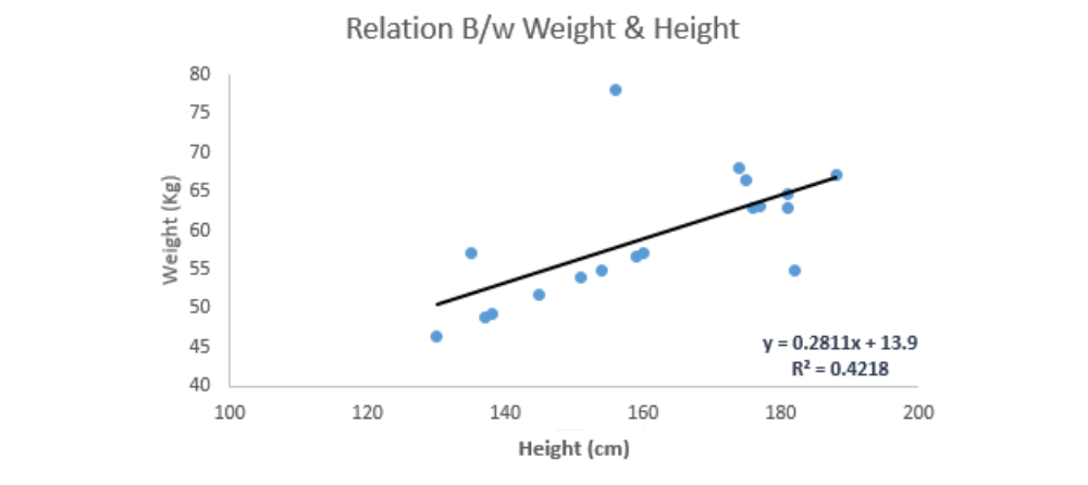
一、线性回归(Linear Regression) 线性回归是用连续变量来估计实际值(房屋成本、通话次数、总销售额等),通过拟合一条最佳的线来建立自变量和因变量之间的关系,这个最佳拟合线称为回归线,用线性方程y = a*x + b表示。1
2
3
4
5
6
7
8
9
10
11
12
13
14
15
16
17
18
from sklearn import linear_model
x_train=input_variables_values_training_datasets
y_train=target_variables_values_training_datasets
x_test=input_variables_values_test_datasets
linear = linear_model.LinearRegression()
linear.fit(x_train, y_train)
linear.score(x_train, y_train)
print ('Coefficient: \n' , linear.coef_)
print ('Intercept: \n' , linear.intercept_)
predicted= linear.predict(x_test)
R代码1
2
3
4
5
6
7
8
9
10
11
x_train <- input_variables_values_training_datasets
y_train <- target_variables_values_training_datasets
x_test <- input_variables_values_test_datasets
x <- cbind(x_train,y_train)
linear <- lm(y_train ~ ., data = x)
summary(linear)
predicted= predict(linear,x_test)
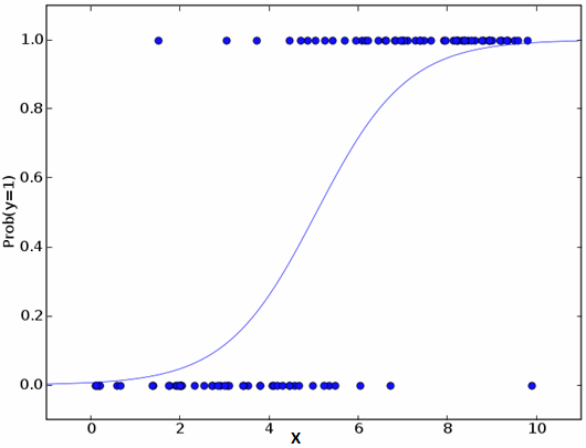
二、逻辑回归(Logistic Regression) 不要被它的名字混淆!它是一种分类而不是回归算法。它是用来估计基于给定自变量集的离散值(二进制值,如0/1,是/否,真/假)。简单地说,它通过将数据拟合到对数函数来预测事件发生的概率,因此,它也被称为对数回归。由于它预测了概率,其输出值介于0和1之间。1
2
3
odds = p/ (1-p) 【事件发生可能性 / 事件发生可能性】
ln(odds) = ln(p/(1-p))
logit(p) = ln(p/(1-p)) = b0 + b1X1 + b2X2 + b3X3 + ... + bkXk
如上,P是存在目标特征的概率,它选择观察样本值的最大似然参数,而不选择普通回归中最小平方误差和。1
2
3
4
5
6
7
8
9
10
11
12
13
from sklearn.linear_model import LogisticRegression
model = LogisticRegression()
model.fit(X, y)
model.score(X, y)
print ('Coefficient: \n' , model.coef_)
print ('Intercept: \n' , model.intercept_)
predicted= model.predict(x_test)
R代码1
2
3
4
5
6
x <- cbind(x_train,y_train)
logistic <- glm(y_train ~ ., data = x,family='binomial' )
summary(logistic)
predicted= predict(logistic,x_test)
除此之外,为了改进模型,还可以尝试更多不同的步骤:包括交互项、去除特征、正则化、使用非线性模型。
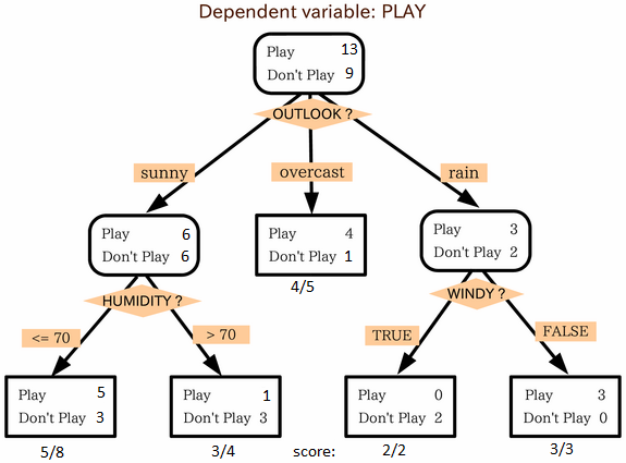
三、决策树(Decision Tree) 决策树是一种主要用于分类问题的监督学习算法,它适用于分类和连续因变量。在该算法中,我们将种群分成两个或更多的同质集,采用关键属性/自变量来尽可能区分的不同组。简化的决策树算法版本 1
2
3
4
5
6
7
8
9
10
11
12
from sklearn import tree
model = tree.DecisionTreeClassifier(criterion='gini' )
model.fit(X, y)
model.score(X, y)
predicted= model.predict(x_test)
R代码1
2
3
4
5
6
7
library(rpart)
x <- cbind(x_train,y_train)
fit <- rpart(y_train ~ ., data = x,method="class" )
summary(fit)
predicted= predict(fit,x_test)
四、SVM (Support Vector Machine) SVM是一种分类方法。在该算法中,我们将每个数据项绘制为n维空间中的一个点(其中n是具有的特征数),其中每个特征的值是特定坐标的值。支持向量机的简化版本 1
2
3
4
5
6
7
8
9
10
from sklearn import svm
model = svm.svc()
model.fit(X, y)
model.score(X, y)
predicted= model.predict(x_test)
R代码1
2
3
4
5
6
7
library(e1071)
x <- cbind(x_train,y_train)
fit <-svm(y_train ~ ., data = x)
summary(fit)
predicted= predict(fit,x_test)
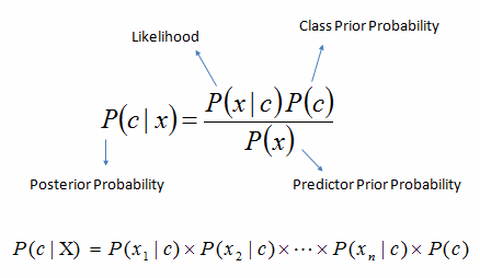
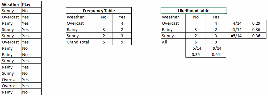
五、朴素贝叶斯 朴素贝叶斯是一种基于贝叶斯定理的分类算法,具有预测属性之间的独立性假设。简单地说,朴素贝叶斯分类器假定类中的特定特征的存在与任何其他特征的存在无关。例如,如果一个水果是红色的、圆的、直径约3英寸的,它可以被认为是一个苹果。即使这些特征彼此依赖或存在其他特征,朴素贝叶斯分类器也认为所有这些属性对“这种水果是苹果”贡献的概率是独立的。 P(Yes) / P (Sunny) 0.64 / 0.36 = 0.60,具有较高的概率。1
2
3
4
5
6
7
8
from sklearn.naive_bayes import GaussianNB
model.fit(X, y)
predicted= model.predict(x_test)
R代码1
2
3
4
5
6
7
library(e1071)
x <- cbind(x_train,y_train)
fit <-naiveBayes(y_train ~ ., data = x)
summary(fit)
predicted= predict(fit,x_test)
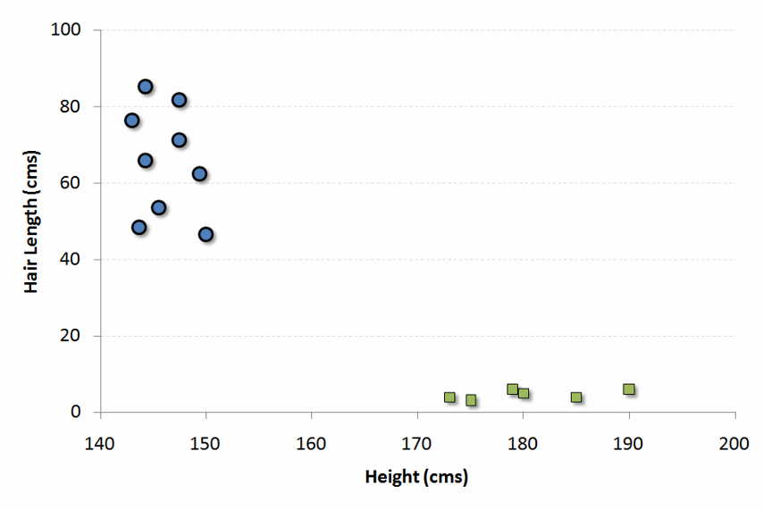
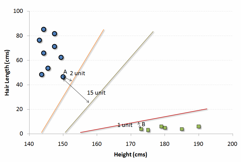
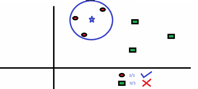
六、kNN (k- Nearest Neighbors) KNN可以用于分类和回归问题,而在工业上常用在分类问题上。K近邻算法是一种简单的算法,它存储了所有可用的样本,并通过其k领域的多数表决对新的样本进行分类。样本的分类是K近邻范围内所有点通过距离函数测量的多数共识。1
2
3
4
5
6
7
8
9
from sklearn.neighbors import KNeighborsClassifier
KNeighborsClassifier(n_neighbors=6)
model.fit(X, y)
predicted= model.predict(x_test)
R代码1
2
3
4
5
6
7
library(knn)
x <- cbind(x_train,y_train)
fit <-knn(y_train ~ ., data = x,k=5)
summary(fit)
predicted= predict(fit,x_test)
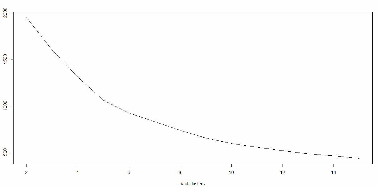
七、K-Means K-Means是一种解决聚类问题的无监督算法。它的过程遵循一种简单且容易的方式,通过一定数量的簇(给定k簇)对给定的数据集进行分类。集群内的数据点对于每组是同质的和异质的。1
2
3
4
5
6
7
8
9
from sklearn.cluster import KMeans
k_means = KMeans(n_clusters=3, random_state=0)
model.fit(X)
predicted= model.predict(x_test)
R代码1
2
library(cluster)
fit <- kmeans(X, 3)
八、随机森林 随机森林是一个包含多个决策树的分类器,它是决策树的集合(被称为“森林”)。为了根据属性对新对象进行分类,每个树都给出分类,并称树为该类“投票”,森林选择选票最多的分类(遍及森林中的所有树)。随机森林简介 CART模型与随机森林的比较(第1部分) 随机森林与CART模型的比较(第2部分) 调整随机森林模型的参数 1
2
3
4
5
6
7
8
9
from sklearn.ensemble import RandomForestClassifier
model= RandomForestClassifier()
model.fit(X, y)
predicted= model.predict(x_test)
R代码1
2
3
4
5
6
7
library(randomForest)
x <- cbind(x_train,y_train)
fit <- randomForest(Species ~ ., x,ntree=500)
summary(fit)
predicted= predict(fit,x_test)
九、降维算法 在过去的4-5年中,数据捕获在每一个可能的阶段都呈指数增长。企业/政府机构/研究机构不仅不断地有新的资源出现,而且还要非常详细地捕捉数据。学习降维算法初学者指南 ”。1
2
3
4
5
6
7
8
9
10
11
from sklearn import decomposition
train_reduced = pca.fit_transform(train)
test_reduced = pca.transform(test )
R代码1
2
3
4
library(stats)
pca <- princomp(train, cor = TRUE)
train_reduced <- predict(pca,train)
test_reduced <- predict(pca,test )
十、梯度提升算法 十点一、GBM GBM是一种利用大量数据进行预测的Boosting算法(Boosting算法是一种用来提高弱分类算法准确度的方法),具有很高的预测能力。实际上,Boosting是学习算法的一种综合,它结合了多个基估计的预测,以提高单个估计器的鲁棒性。它将多个弱预测因子或平均预测因子组合成一个强预测因子。这些Boosting算法在Kaggle、AV Hakason、CrowdAnalytix等数据科学竞赛中有很好。详细了解Boosting算法 1
2
3
4
5
6
7
8
9
from sklearn.ensemble import GradientBoostingClassifier
model= GradientBoostingClassifier(n_estimators=100, learning_rate=1.0, max_depth=1, random_state=0)
model.fit(X, y)
predicted= model.predict(x_test)
R代码1
2
3
4
5
6
library(caret)
x <- cbind(x_train,y_train)
fitControl <- trainControl( method = "repeatedcv" , number = 4, repeats = 4)
fit <- train(y ~ ., data = x, method = "gbm" , trControl = fitControl,verbose = FALSE)
predicted= predict(fit,x_test,type = "prob" )[,2]
梯度提升分类器和随机森林是两种不同的提升树分类器,两种算法间的差异 。
十点二、XGBoost 另一种经典的梯度提升算法通常是一些Kaggle比赛中成败的决定性选择。点这里 。1
2
3
4
5
6
7
8
9
10
11
from xgboost import XGBClassifier
from sklearn.model_selection import train_test_split
from sklearn.metrics import accuracy_score
X = dataset[:,0:10]
Y = dataset[:,10:]
seed = 1
X_train, X_test, y_train, y_test = train_test_split(X, Y, test_size=0.33, random_state=seed)
model = XGBClassifier()
model.fit(X_train, y_train)
y_pred = model.predict(X_test)
R代码1
2
3
4
5
6
7
8
require(caret)
x <- cbind(x_train,y_train)
TrainControl <- trainControl( method = "repeatedcv" , number = 10, repeats = 4)
model<- train(y ~ ., data = x, method = "xgbLinear" , trControl = TrainControl,verbose = FALSE)
OR
model<- train(y ~ ., data = x, method = "xgbTree" , trControl = TrainControl,verbose = FALSE)
predicted <- predict(model, x_test)
十点三、LightGBM LightGBM是一种使用基于树的学习算法的梯度提升框架。它被设计成分布式的、高效的,优点如下:点这里 。1
2
3
4
5
6
7
8
9
10
11
12
data = np.random.rand(500, 10)
label = np.random.randint(2, size=500)
train_data = lgb.Dataset(data, label=label)
test_data = train_data.create_valid('test.svm' )
param = {'num_leaves' :31, 'num_trees' :100, 'objective' :'binary' }
param['metric' ] = 'auc'
num_round = 10
bst = lgb.train(param, train_data, num_round, valid_sets=[test_data])
bst.save_model('model.txt' )
data = np.random.rand(7, 10)
ypred = bst.predict(data)
R代码1
2
3
4
5
6
7
8
9
10
11
12
13
14
15
16
17
library(RLightGBM)
data(example.binary)
num_iterations <- 100
config <- list(objective = "binary" , metric="binary_logloss,auc" , learning_rate = 0.1, num_leaves = 63, tree_learner = "serial" , feature_fraction = 0.8, bagging_freq = 5, bagging_fraction = 0.8, min_data_in_leaf = 50, min_sum_hessian_in_leaf = 5.0)
handle.data <- lgbm.data.create(x)
lgbm.data.setField(handle.data, "label" , y)
handle.booster <- lgbm.booster.create(handle.data, lapply(config, as.character))
lgbm.booster.train(handle.booster, num_iterations, 5)
pred <- lgbm.booster.predict(handle.booster, x.test)
sum(y.test == (y.pred > 0.5)) / length(y.test)
lgbm.booster.save(handle.booster, filename = "/tmp/model.txt" )
如果您熟悉R中的Caret包的话,以下是实现LightGBM的另一种方式:1
2
3
4
5
6
7
8
9
10
11
12
13
require(caret)
require(RLightGBM)
data(iris)
model <-caretModel.LGBM()
fit <- train(Species ~ ., data = iris, method=model, verbosity = 0)
print (fit)
y.pred <- predict(fit, iris[,1:4])
library(Matrix)
model.sparse <- caretModel.LGBM.sparse()
mat <- Matrix(as.matrix(iris[,1:4]), sparse = T)
fit <- train(data.frame(idx = 1:nrow(iris)), iris$Species , method = model.sparse, matrix = mat, verbosity = 0)
print (fit)
十点四、Catboost Catboost是最近从Yandex开源的机器学习算法,它可以很容易地与谷歌的TensorFlow和苹果的Core ML等深度学习框架相结合。从这篇文章 。1
2
3
4
5
6
7
8
9
10
11
12
13
14
15
16
17
18
19
20
21
22
import pandas as pd
import numpy as np
from catboost import CatBoostRegressor
train = pd.read_csv("train.csv" )
test = pd.read_csv("test.csv" )
train.fillna(-999, inplace=True)
test.fillna(-999,inplace=True)
X = train.drop(['Item_Outlet_Sales' ], axis=1)
y = train.Item_Outlet_Sales
from sklearn.model_selection import train_test_split
X_train, X_validation, y_train, y_validation = train_test_split(X, y, train_size=0.7, random_state=1234)
categorical_features_indices = np.where(X.dtypes != np.float)[0]
from catboost import CatBoostRegressormodel=CatBoostRegressor(iterations=50, depth=3, learning_rate=0.1, loss_function='RMSE' )
model.fit(X_train, y_train,cat_features=categorical_features_indices,eval_set=(X_validation, y_validation),plot=True)
submission = pd.DataFrame()
submission['Item_Identifier' ] = test ['Item_Identifier' ]
submission['Outlet_Identifier' ] = test ['Outlet_Identifier' ]
submission['Item_Outlet_Sales' ] = model.predict(test )
R代码1
2
3
4
5
6
7
8
9
10
11
12
13
14
set.seed(1)
require(titanic)
require(caret)
require(catboost)
tt <- titanic::titanic_train[complete.cases(titanic::titanic_train),]
data <- as.data.frame(as.matrix(tt), stringsAsFactors = TRUE)
drop_columns = c("PassengerId" , "Survived" , "Name" , "Ticket" , "Cabin" )
x <- data[,!(names(data) %in % drop_columns)]y <- data[,c("Survived" )]
fit_control <- trainControl(method = "cv" , number = 4,classProbs = TRUE)
grid <- expand.grid(depth = c(4, 6, 8),learning_rate = 0.1,iterations = 100, l2_leaf_reg = 1e-3, rsm = 0.95, border_count = 64)
report <- train(x, as.factor(make.names(y)),method = catboost.caret,verbose = TRUE, preProc = NULL,tuneGrid = grid, trControl = fit_control)
print (report)
importance <- varImp(report, scale = FALSE)
print (importance)
至止,你将对常用的机器学习算法有所了解。